The Support Vector Machine (SVM) is a linear classifier that can be viewed as an extension of the Perceptron developed by Rosenblatt in 1958. The Perceptron guaranteed that you find a hyperplane if it exists. The SVM finds the maximum margin separating hyperplane.

In addition to performing linear classification:

\[f(x)= sign(\mathbf{w^Tx}+b)= \begin{cases} +1 & \text{if $\mathbf{w^Tx}+b>0$}\\ -1 & \text{if $\mathbf{w^Tx}+b \leq 0$}\end{cases}\]

SVMs can efficiently perform a non-linear classification using what is called the kernel trick, implicitly mapping their inputs into high-dimensional feature spaces.[1]

An hyperplane is defined as the points such that $\mathbf{w}^T \mathbf{x} + b = 0$.

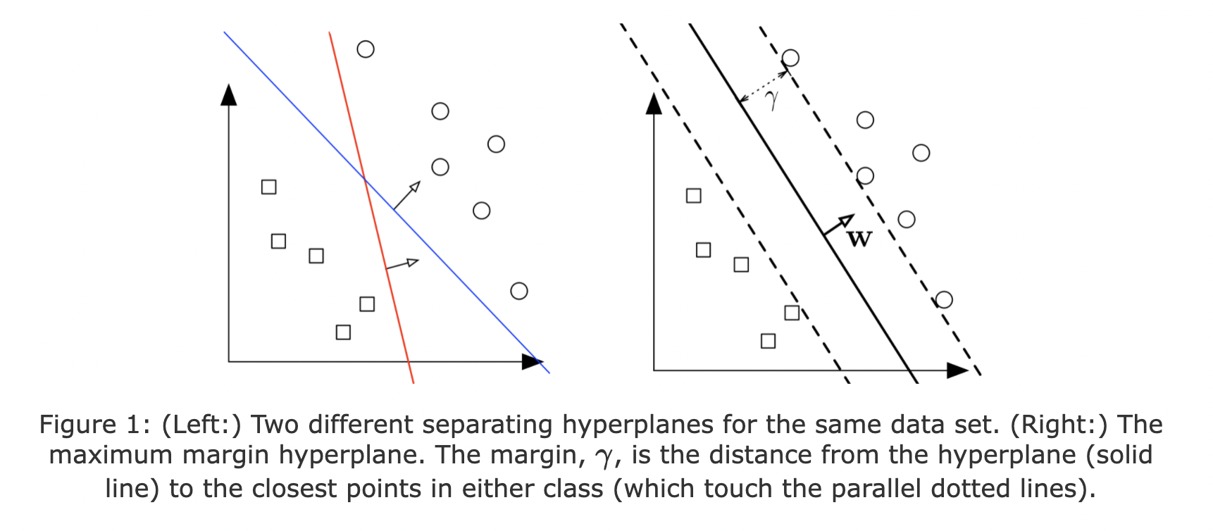
Given a training dataset of $n$ points of the form $(\mathbf{x}_1,y_{1}),\ldots ,(\mathbf{x}_n,y_{n})$ where the $y_{i}$ are either 1 or −1, , each indicating the class to which the point $\mathbf{x}_i$ belongs. We want to find the “maximum-margin hyperplane” that divides the group of points $\mathbf{x}_i$ for which $y_i=1$ from the group of points for which $y_i=-1$, a binary linear classifier of the form of $\mathbf{w}^T \mathbf{x} + b = 0$. What is the best separating hyperplane? SVM Answer: The one that maximizes the distance to the closest data points from both classes. We say it is the hyperplane with maximum margin.

My helpful screenshot

Margin

Let the margin $\gamma$ be defined as the distance of the closest $\mathbf{x}$ from the hyperplane $H=\{\mathbf{x|w^Tx}+b=0\}$

Margin of $H$ with respect to $D$: $\gamma(\mathbf{w},b)= \min_{\mathbf{x} \in D} \frac{\mathbf{w^Tx}+b}{||\mathbf{x}||_2}$

What is the general distance of a point $\mathbf{x}$ to the hyperplane $H$?

If we define the following elements: the hyperplane $H$, a point $\mathbf{x}$ in the space close to the hyperplane, $\mathbf{x_P}$ its projection on the hyperplane, and $\mathbf{\overrightarrow{d}}$ as the distance vector from $\mathbf{x_P}$ to $\mathbf{x}$.

My helpful screenshot

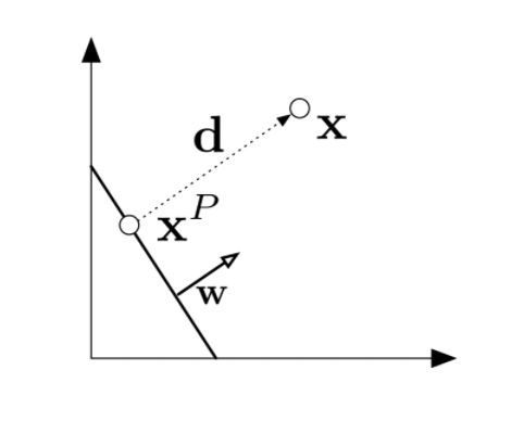
It will follow that to calculate the distance $\mathbf{d}$

\[\mathbf{x_P} = \mathbf{x} - \mathbf{d}\] \[\mathbf{d} \quad \textrm{is parallel to} \quad \mathbf{w}\quad , \textrm{so } \quad \mathbf{d}=\alpha \mathbf{w} \quad\textrm{for some } \alpha \in R\] \[\mathbf{x_P} \in \textrm{H which implies} \quad \mathbf{w^Tx_P} + b = 0\] \[\textrm{therefore} \quad \mathbf{w^Tx_P} + b = \mathbf{w^T(x−d)} + b = \mathbf{w^T(x−αw)} + b = 0\] \[\textrm{which implies } \quad\alpha = \frac{\mathbf{w^Tx}+b}{\mathbf{w^Tw}}\]

The length of $\mathbf{d}$:

\[||\mathbf{d}||_2 = \sqrt{\mathbf{d^Td}} = \sqrt{\alpha^2\mathbf{w^Tw}} = \frac{∣\mathbf{w^Tx}+b∣}{\sqrt{\mathbf{w^Tw}}} = \frac{∣\mathbf{w^Tx}+b∣}{||w||_2}\]

Margin of $H$ with respect to $D$: $\gamma(\mathbf{w},b)= \min_{\mathbf{x} \in D} \frac{\mathbf{w^Tx}+b}{||\mathbf{w}||_2}$

Note that if the hyperplane is such that γ is maximized, it must lie right in the middle of the two classes.

Maximizing margins, constrained formulation: hard margins

By constrained or hard margine we mean that our objective is to maximize the margin under the constraints that all data points must lie on the correct side of the hyperplane:

$\textrm{Maximize margin} \quad \max_{\mathbf{w},b} \gamma(\mathbf{w},b)$ $\textrm{such that} \quad \forall_i \quad y_i(\mathbf{w^Tx_i}+b) \geq 0$

By plugging in the definition of $\gamma$ we obtain:

$\max_{\mathbf{x},b} \frac{1}{||\mathbf{w}||_2} \min_{\mathbf{x} \in D} |\mathbf{w^Tx_i}+b|$ $\textrm{such that} \quad \forall_i \quad y_i(\mathbf{w^Tx_i}+b) \geq 0$

Because the hyperplane is scale invariant, we can fix the scale of $\mathbf{w},b$ anyway we want. Let’s be clever about it, and choose it such that

\[\min_{\mathbf{x} \in D} |\mathbf{w^Tx}+b| = 1\]

Then our maximization function becomes easier:

\[\max_{\mathbf{x},b} \frac{1}{||\mathbf{w}||_2} \cdot 1 = \min_{\mathbf{w},b} \mathbf{w^Tw}\]

The new optimization problems becomes:

\[\min_{\mathbf{w},b} \mathbf{w^Tw}\]

such that:

$\quad \forall_i \quad y_i(\mathbf{w^Tx_i}+b) \geq 0$ $\min_{i} |\mathbf{w^Tx_i}+b| = 1$

or equivalently: $\min_{\mathbf{w},b} \mathbf{w^Tw}$

such that:

\[\forall_i \quad y_i(\mathbf{w^Tx_i}+b) \geq 1\]

Support vectors

Support vectors are the data points that lie closest to the decision surface (or hyperplane), they have direct bearing on the optimum location of the decision surface.

For the optimal $\mathbf{w},b$ pair, some training points will have tight constraints, i.e.

\[\quad y_i(\mathbf{w^Tx_i}+b) = 1\]

We refer to these training points as support vectors. Support vectors are special because they are the training points that define the maximum margin of the hyperplane to the data set and they therefore determine the shape of the hyperplane.

Unconstrained formulation: soft margins

When data are non-linearly separable, we can not find an hyperplane, so we can not obtain a solution from the SVM optimization problem.

We can allow the constraints to be violated, following this formulation:

\[\min_{\mathbf{w},b} \mathbf{w^tw} + c \sum_{i=1}^n \xi_i\] \[\textrm{s. t.} \forall_i \quad y_i(\mathbf{w^Tx_i}+b) \geq 1 - \xi_i\] \[\forall_i \quad \xi_i \geq 0\]

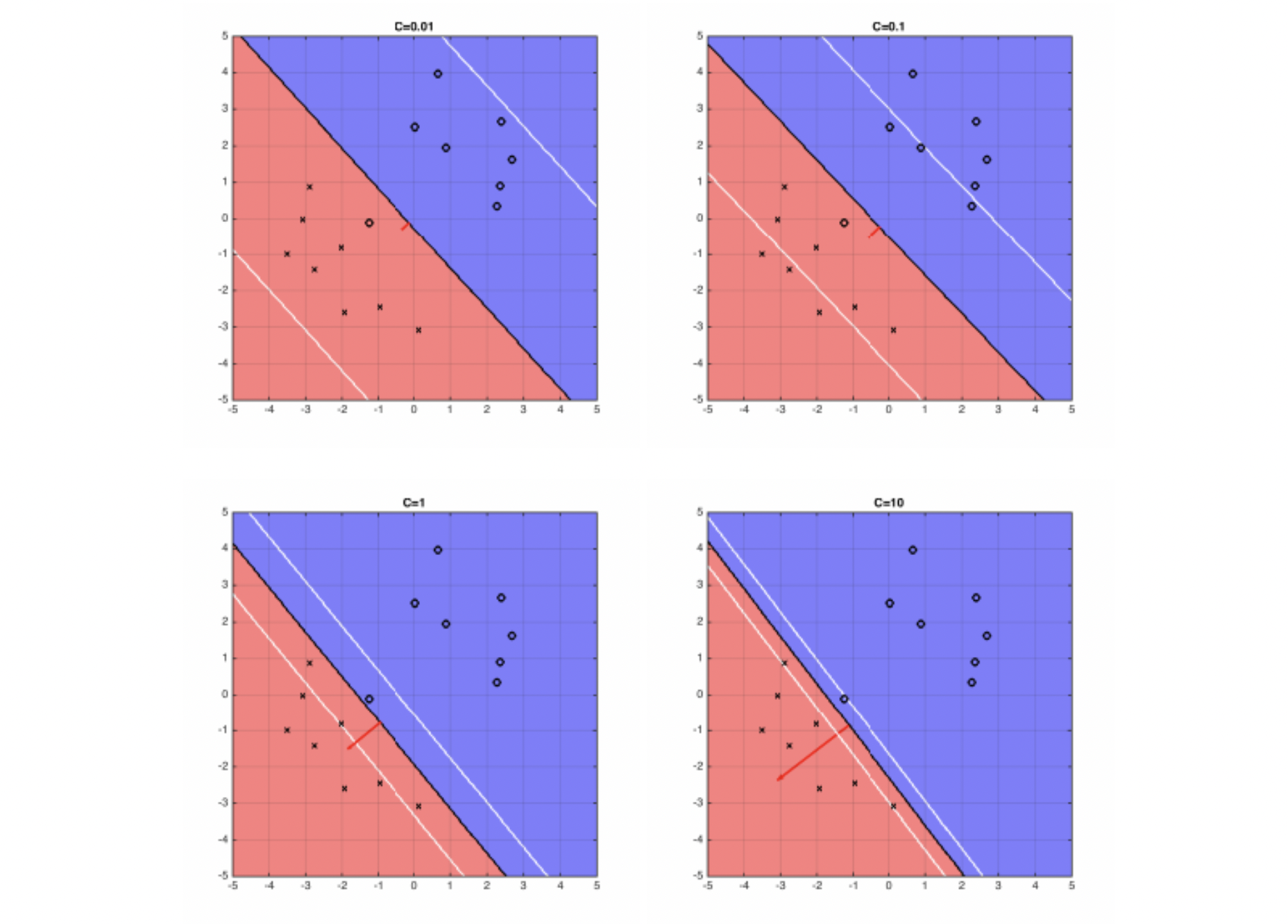
$\xi_i$ is called slack variable and allows the data points $\mathbf{x_i}$ to be closer to the hyperplane or even cross it when C is very small.

If C is very large, the SVM becomes very strict and tries to get all points to be on the right side of the hyperplane
If C is very small, the SVM becomes very loose and may “sacrifice” some points to obtain a simpler solution (i.e. lower $||\mathbf{w}||_2^2$ )

Formulation:

\[\xi_i= \begin{cases} 1 - y_i(\mathbf{w^Tx_i}+b) \leq 1 & \quad \textrm{if} \quad y_i(\mathbf{w^Tx_i}+b) <1\\ 0 & \quad \textrm{if} \quad y_i(\mathbf{w^Tx_i}+b) \geq 1\end{cases}\]

Equivalent to:

\[\xi_i = max(1-y_i(\mathbf{w^Tx_i}+b),0)\]

If we plug this closed form in the objective of the SVM optimization problem we obtain:

\[\min_{\mathbf{w},b} \mathbf{w^Tw} + C \sum_{i=1}^n max[1-y_i(\mathbf{w^Tx_i}+b),0]\]

The four plots below show different boundary of hyperplane and the optimal hyperplane separating example data, when $C=0.01, 0.1, 1, 10$.

My helpful screenshot

Risk minimization

Recalling the SVM optimization problem

\[\min_{\mathbf{w}} \quad C\underbrace{\sum_{i=1}^n max[1-y_i(\mathbf{w^Tx_i}+b),0]}_{Hinge-Loss} + \underbrace{\mathbf{w^Tw}}_\text{Regularizer}\]

This formulation can be generalized:

\[\min_{\mathbf{w}} \quad \frac{1}{n} \sum_{i=1}^n \underbrace{l(h_{\mathbf{w}}(\mathbf{x_i}),y_i }_\text{Loss} + \underbrace{\lambda r(\mathbf{w})}_{Regularizer}\]

where the Loss Function is a continuous function that penalizes the error and the Regularizer pensalizes the model complexity.

Risk minimization: Loss functions

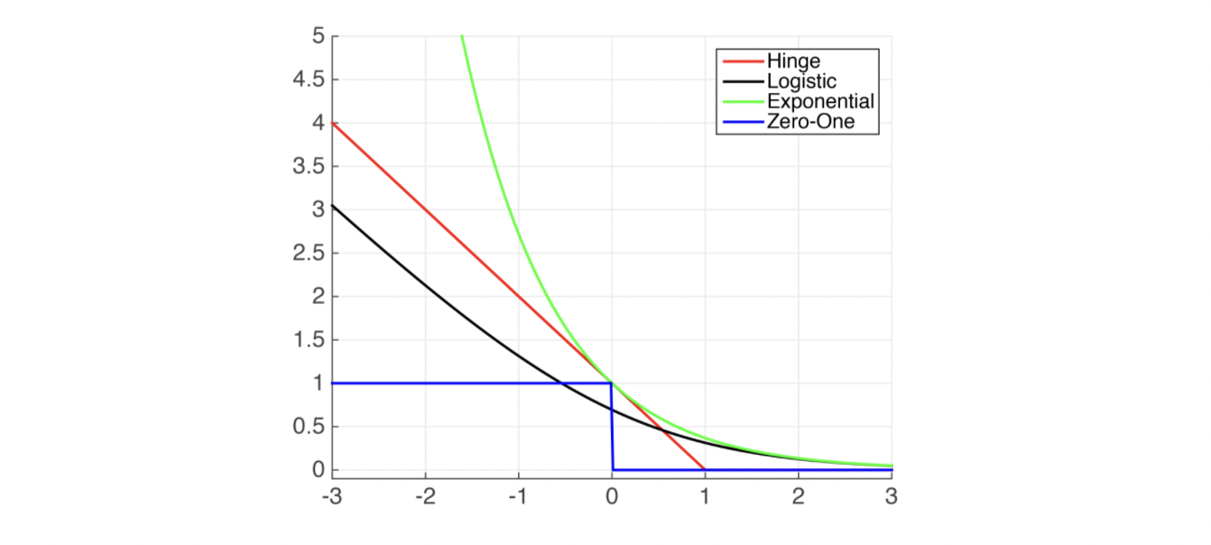
Common Binary Classification Loss functions

Hinge Loss: $max[1-y_i(\mathbf{w^Tx_i}+b),0]^P$

Used in Standard SVM $p=1$

Comments: When used for Standard SVM, the loss function denotes the size of the margin between linear separator and its closest points in either class. Only differentiable everywhere with $p=2$.

Log-Loss: $log(1+e^{-h_w(x_i)y_i})$

Used in Logistic Regression

Comments: Popular in machine learning

Explonential Loss: $e^{-h_w(x_i)y_i}$

Used in AdaBoost

Comments: This function is very aggressive. The loss of a mis-prediction increases exponentially with the value of $-h_w(x_i)y_i$. This can lead to nice convergence results, for example in the case of Adaboost, but it can also cause problems with noisy data.

Zero-One Loss: $\delta(sign(h_w(x_i))\neq y_i)$

Used in Actual Classification Loss

Comments: Non-continuous and thus impractical to optimize.

Plots of Common Classification Loss Functions: My helpful screenshot

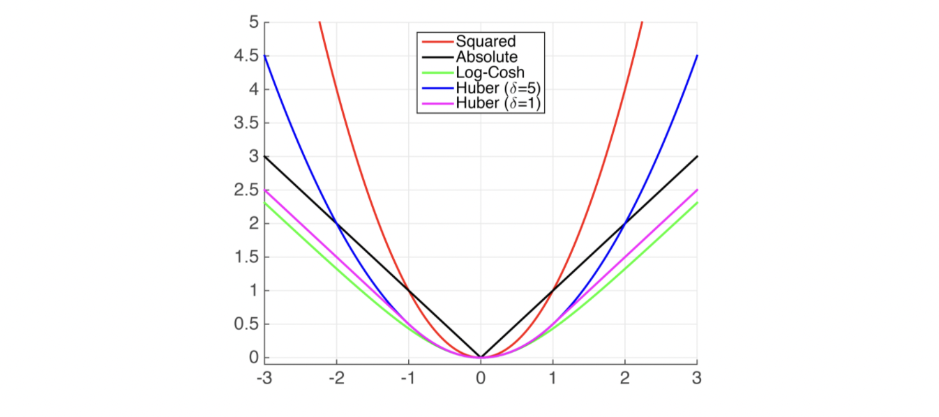
Common Regression Loss functions

Squared Loss: $(h(x_i)-y_i)^2$

Comments: Also known as Ordinary Least Squares (OLS)

Absolute Loss: $|h(x_i)-y_i|$

Comments: Less sensitive to noise but not differentiable at $0$

Huber Loss: $H= \begin{cases} \frac{1}{2}(h\mathbf({x_i})-y_i)^2 & \quad \textrm{if} \quad |h\mathbf({x_i})-y_i| < \delta\\ \delta(|h\mathbf({x_i})-y_i|-\frac{\delta}{2}) & \quad \textrm{otherwise}\end{cases}$

Comments: Takes on behavior of Squared-Loss when loss is small, and Absolute Loss when loss is large.

Plots of Common Regression Loss Functions: My helpful screenshot

Risk minimization: Regularizers

Now the optimization problem formulation:

\[\min_{\mathbf{w},b} \quad \sum_{i=1}^n l(h_{\mathbf{w}}(\mathbf{x}),y_i) + \lambda r(\mathbf{w})\]

should be changed to this one:

\[\min_{\mathbf{w},b} \quad \sum_{i=1}^n l(h_{\mathbf{w}}(\mathbf{x}),y_i) \quad \textrm{subject to} \quad r(\mathbf{w}) \leq B\]

L2 Regularizer: $r(\mathbf{w})=\mathbf{w}^T\mathbf{w}=||\mathbf{w}||_2^2$

Comments: Strictly convex, differentiable

L1 Regularizer: $r(\mathbf{w})=||\mathbf{w}||_1$

Comments: Not differentiable at $0$

LP Norm: $||\mathbf{w}||_P = \sum_{i=1}^{d} (v_i^p)^{\frac{1}{p}}$

References:

Support-vector machines, Wikipedia, https://en.wikipedia.org/wiki/Support-vector_machine
Machine Learning for Intelligent Systems, Kilian Weinberger, Cornell University, https://www.cs.cornell.edu/courses/cs4780/2018fa/page18/
Application of SVM, Jakevdp, https://jakevdp.github.io/PythonDataScienceHandbook/05.07-support-vector-machines.html