Naïve Bayes Classifiers
Introduction
Naive Bayes is a simple technique for constructing classifiers that can detect the class labels to problem instances. Let us assume that a single problem instance \(\mathbf{x}= (x_{1},\ldots ,x_{n})\) is given and represented as vectors of feature values, we are interested in predicting another characteristic \(C_k\), which can take on K possible values. There is not a single algorithm for training such classifiers, but a family of algorithms based on a common principle: all naive Bayes classifiers assume that the value of a particular feature is independent of the value of any other feature, given the class variable. For example, a fruit may be considered to be an apple if it is red, round, and about 10 cm in diameter. A naive Bayes classifier considers each of these features to contribute independently to the probability that this fruit is an apple, regardless of any possible correlations between the color, roundness, and diameter features.[1]
Probabilistic model
Given a problem instance to be classified, represented by a vector \(\mathbf{x} = (x_{1},\ldots ,x_{n})\) representing some n features (independent variables), for each of \(K\) possible outcomes or classes \(C_k\), it assigns to this instance class conditional probability:
\[P(C_k | x_{1},\ldots ,x_{n}) = P(C_k | \mathbf{x})\]Using Bayes’ theorem, the conditional probability can be decomposed into the product of the likelihood and the prior scaled by the likelihood of the data:
\[P(C_k | \mathbf{x}) = \frac{P(C_k)P(\mathbf{x}|C_k)}{P(\mathbf{x})}\] \[posterior = \frac{prior \times likelihood}{evidence}\]Since the random variables \(\mathbf{x} = (x_{1},\ldots ,x_{n})\) are (naïvely) assumed to be conditionally independent, given the class label Ck, the likelihood on the right-hand side can be simply re-written as:
\[P(C_k | x_{1},\ldots ,x_{n}) = \frac{P(C_k) \prod_{i=1}^n P(x_i | C_k)}{P(x_1, \ldots, x_n)}\]Since the denominator \(P(x_1, \ldots, x_n)\) is a constant with respect to the class label \(C_k\), the conditional probability is proportional to the numerator:
\[P(C_k | x_{1},\ldots ,x_{n}) \propto P(C_k) \prod_{i=1}^n P(x_i | C_k)\]In order to avoid a numerical underflow (when n » 0), these calculations are performed on the log scale:
\[log[P(C_k | x_{1},\ldots ,x_{n})] \propto log[P(C_k)] + \sum_{i=1}^n log[P(x_i | C_k)]\]The classifier, is the function that finds the class label \(\hat{C_k}\) for some K with the highest log-posterior probability:
\[\hat{C} = argmax_{k} log[P(C_k | x_{1},\ldots ,x_{n})] \propto log[P(C_k)] + \sum_{i=1}^n log[P(x_i | C_k)]\]The classifier algorithm is already implemented in out of the box functions.
Prior distribution
A class’s prior probability \(P(C_k)\) may be calculated:
- by assuming equiprobable classes (i.e., \(P(C_{k})=\frac{1}{K}\))
- by calculating an estimate for the class probability from the training set (i.e., prior for a given class = number of samples in the class/total number of samples)
- by manually specifying an arbitrary value
Assumptions on the distribution of the features \(x_i\)
Each individual feature \(x_i\) can take a value from a finite/infinte set of m individually identified items (discrete feature) or it can be any real valued number (continuous feature). Depending on the kind of the feature \(x_i\), the naivebayes() function uses a different probability distribution for modelling of the class conditional probability
\(P(x_i | C_k)\).
-
Continuous data (Gaussian Naïve Bayes)
When dealing with continuous features, a typical assumption is that the values associated with each class are distributed according to a normal (or Gaussian) distribution. For example, suppose the training data contains a continuous attribute, \(X_i\). The data is first segmented by the class, and then the mean and variance of \(X_i\) is computed in each class. Let \(\mu_{ik}\) be the mean of the values in \(X_i\) associated with class \(C_{k}\), and let \(\sigma_{ik}^2\) be the corrected variance of the values in \(X_i\) associated with class \(C_{k}\). Suppose one has collected some observation value \(v\). Then, the probability density of \(v\) given a class \(C_{k}\), \(p(X_i=v | C_{k})\) can be computed by plugging v into the equation for a normal distribution parameterized by \(\mu _{ik}\) and \(\sigma _{ik}^{2}\). That is:
\[P(X_i=v|C_k)= \frac{1}{\sqrt{2 \pi \sigma_{ik}^2}}e^{-\frac{v-\mu_{ik}}{2 \sigma_{ik}^2}}\]-
Categorical features
If \(X_i\) is discrete feature which takes on M possible values denoted by \(X_i = {item1, ..., itemM}\), then the Categorical distribution is assumed:
\[P(X_i = l| Ck) = p_{ikl}\]where \(p_{ikl} > 0\) and \(\sum_{j \in X_i} pikj = 1\)
-
Binary features (Bernoulli Naïve Bayes)
The Bernoulli distribution is the special case of categorical features for M = 2. It is important to note that the logical (TRUE/FALSE) vectors are internally coerced to character (“TRUE”/”FALSE”) and hence are assumed to be discrete features. Also, if the feature \(x_i\) takes on 0 and 1 values only it would be necessary to transform the variable from numerical to categorical.
\[P( \mathbf{x} | C_k) = \prod_{i=1}^n p_{ki}^{x_i} (1-p_{ki})^{1-x_i}\]where \(p_{ki}\) is the probability of class \(C_{k}\) generating the term \(x_{i}\).
-
Non-negative integer feature (Poisson Naïve Bayes)
If \(x_i\) is a non-negative integer feature and explicitly requested via naive_bayes(..., use- poisson = TRUE) then the Poisson distribution is assumed:
where \(\lambda_{ik} > 0\) and \(v ∈ {0, 1, 2, ...}\). If this applies to all features, then the model can be called a “Poisson Naive Bayes”.
A simple example in R
Using the ”naivebayes” package in R (or any equivalent), let us implement a Naive Bayes Classifier on this dataset, by making the assumption that each feature can be modelled by a Gaussian distribution.
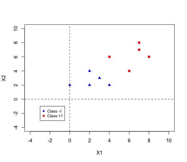 Fig 1 Data [1]
# Initialize the data set
library(naivebayes)
A <- matrix(c(2,2,-1,2,4,-1,4,2,-1,3,3,-1,0,2,-1,
6,4,1,4,6,1,8,6,1,7,7,1,7,8,1),nrow = 10, ncol = 3, byrow = TRUE)

X <- A[,1:2]
Y <-as.factor(A[,3])
colnames(A) <- c("X1", "X2", "Y")

### Train the Gaussian Naive Bayes
gnb <- gaussian_naive_bayes(x = X, y = Y)
summary(gnb)

# Print Parameters
coef(gnb)
print(gnb[[3]])
Running the command “coef(gnb)” or extrapolating the parameters from the “gaussian_naive_bayes” table is the same, and we will obtain the following parameters:
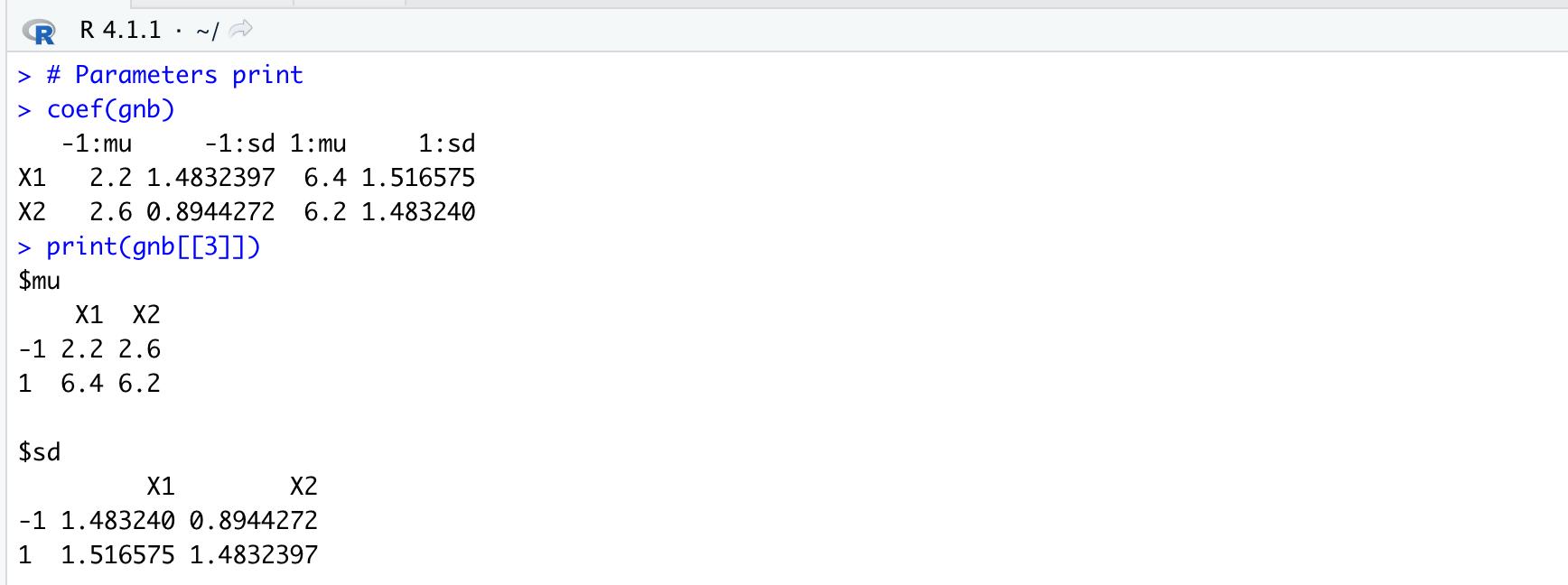 Fig 2 Results [2]
Plot the projections of the data against each feature (1 plot each) and note how these are linked to the values found in the previous question.
# Visualize class conditional densities
plot(gnb, "X1", prob = "conditional")
plot(gnb, "X2", prob = "conditional")
It is immediate to see that the mean for the feature X1 is \(2.2\) for class \(-1\) is \(2.2\) and for class \(+1\) is $6.4$ with respective standard deviation of \(1.48\) and \(1.52\). The mean for the feature X2 is \(2.6\) for class \(-1\) is \(6.2\) and for class \(+1\) is \(6.4\) with respective standard deviation of \(0.89\) and \(1.48\).
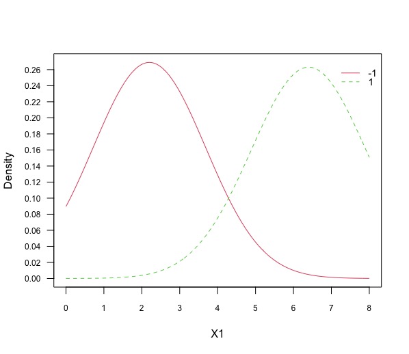 Fig 3 Plot [3]
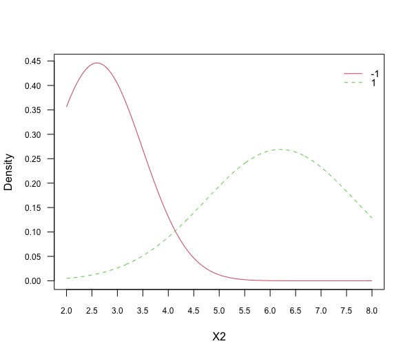 Fig 4 Plot [4]
Predict the label of a test point \(x_{test} = (x1 = 4, x2 = 4)\) and give \(P(y=-1|x_{test})\)
# Set testing data
test <- matrix(c(4,4), nrow = 1, ncol = 2)
colnames(test) <- c("X1", "X2")

# Prediction of the class
C <- predict(gnb, test, type = "class")
print(C)

# Display conditional probability of the class for this data
D <- predict(gnb, test, type = "prob")
print(D[,1])
The predicted label for the \(x_{test}=-1\), while the conditional probability of the class is \(0.714805\)
References:
- Wikipedia, https://en.wikipedia.org/wiki/Naive_Bayes_classifier
- Michal Majka, Introduction to naivebayes package, March 8, 2020